Ridgeline Plot Maker for Comparing Many Distributions

Stack a density curve for every group on one shared axis and see how the distributions shift.

Upload a group column and a numeric column. SciFigure estimates each group’s density with one joint bandwidth, scales every ridge on the same height scale, marks medians, and draws a clean ridgeline plot for months, cell types, sessions, sites, or any other ordered groups.

Up to 20 ridgesJoint KDE bandwidthOverlay two or three conditions

AI Ridgeline Plot Maker

Upload grouped data and describe the plot.

Try sample data

Aspect ratio
283 / 2000 characters

Costs 5 credits. Density curves, medians, and quartiles are computed from your uploaded data, then drawn as a PNG.

Preview

Ridgeline Plot Examples

Aspect ratio: 16:9

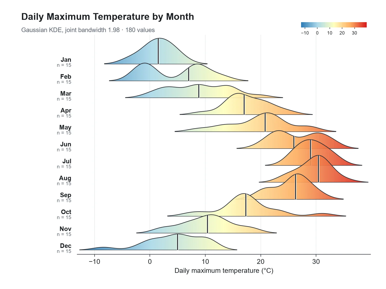
Monthly Temperature Ridgeline Plot ridgeline plot example preview
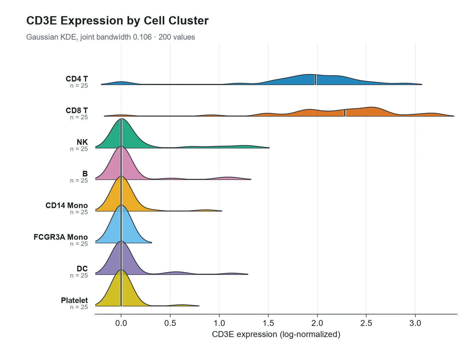
Marker Expression by Cell Cluster ridgeline plot example preview
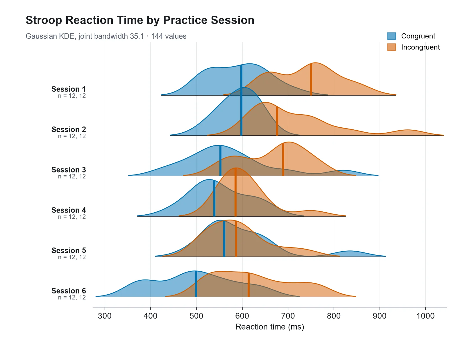
Reaction Time Ridgelines with Two Conditions ridgeline plot example preview

These previews were drawn from the sample datasets. Load a sample or upload your own file to generate a ridgeline plot.

Ridgeline plot examples

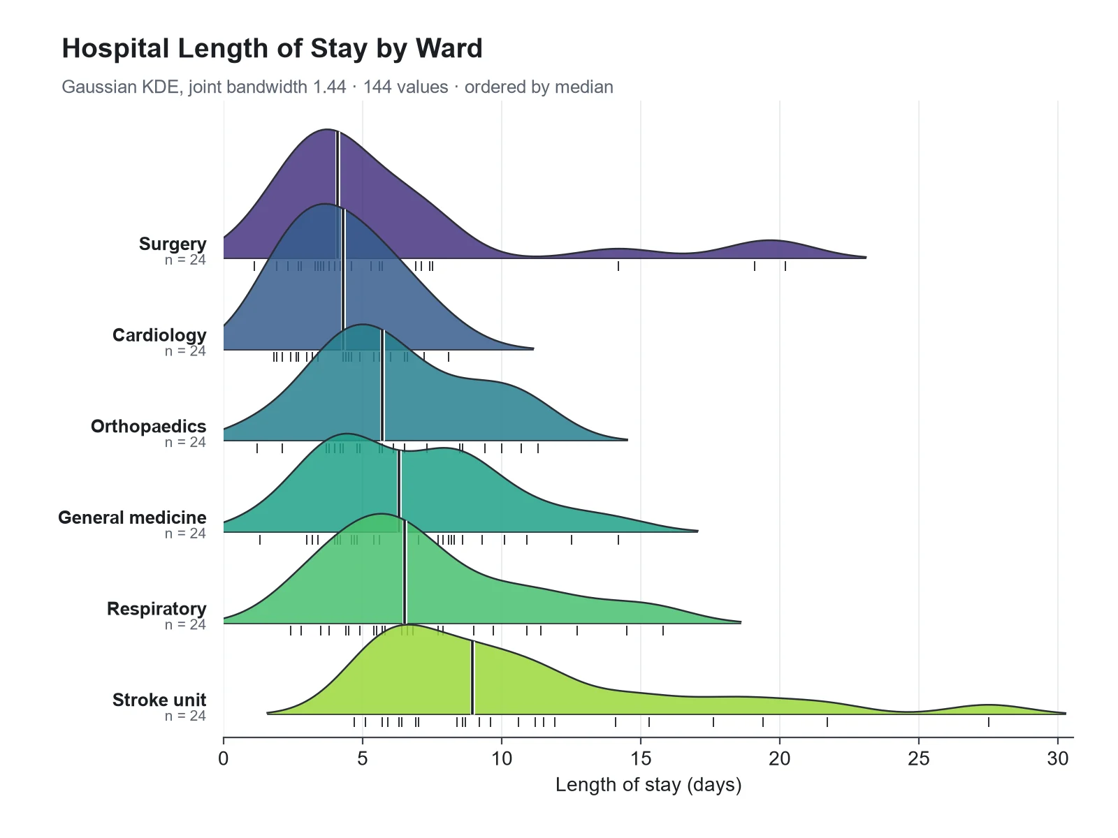
Each example was drawn from a sample dataset: seasonal temperatures, marker expression across single-cell clusters, reaction times with two overlaid conditions, a phenology shift over years, particle sizes by synthesis temperature, and hospital length of stay ordered by median.

Ridgeline Plot Maker: Monthly Temperature Ridgeline Plot scientific chart example

Prompt

Based on the uploaded daily_max_temperature.csv file, create a ridgeline plot of daily maximum temperature by month, January at the top and December at the bottom, ridges filled with a cool-to-warm gradient by temperature, a median line in each ridge, and an overlap of 1.6.
Monthly Temperature Ridgeline Plot

Ridgeline Plot Maker: Marker Expression by Cell Cluster scientific chart example

Prompt

Based on the uploaded pbmc_cd3e_expression.csv file, create a ridgeline plot of CD3E log-normalized expression for each cell cluster, one color per cluster, a median line in each ridge, an overlap of 1.2, and an x-axis label "CD3E expression (log-normalized)". Keep the zero spike visible.

Marker Expression by Cell Cluster

Ridgeline Plot Maker: Reaction Time Ridgelines with Two Conditions scientific chart example

Prompt

Based on the uploaded stroop_sessions.csv file, create a ridgeline plot of reaction time by practice session with congruent and incongruent trials overlaid in each ridge (blue and orange, semi-transparent), an overlap of 1.2, a legend for the two conditions, and median lines.

Reaction Time Ridgelines with Two Conditions

Ridgeline Plot Maker: Flowering Date by Year scientific chart example

Prompt

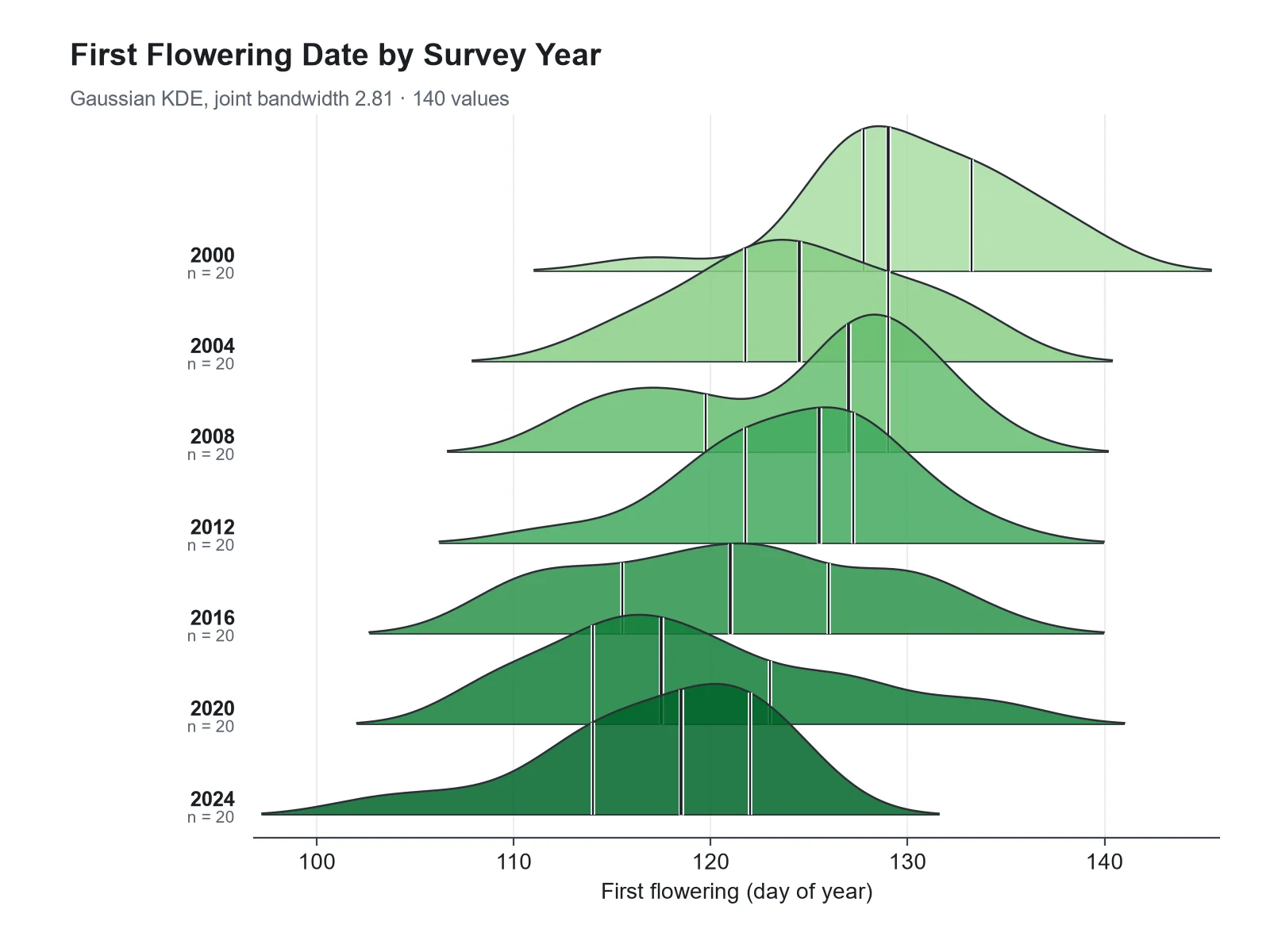
Based on the uploaded flowering_day_of_year.csv file, create a ridgeline plot of first flowering day of year, one ridge per survey year from 2000 at the top to 2024 at the bottom, green fills, median lines, and quartile lines.

Flowering Date by Year

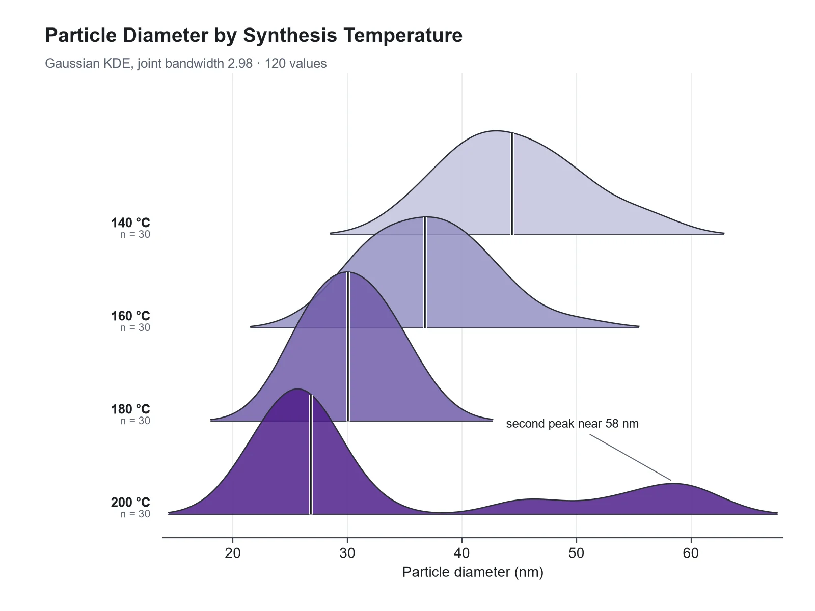
Ridgeline Plot Maker: Nanoparticle Size by Synthesis Temperature scientific chart example

Prompt

Based on the uploaded particle_diameter_dls.csv file, create a ridgeline plot of particle diameter (nm) for each synthesis temperature, a sequential purple palette from low to high temperature, and an annotation of the second peak at 200 °C.

Nanoparticle Size by Synthesis Temperature

Ridgeline Plot Maker: Length of Stay by Ward, Ordered by Median scientific chart example

Prompt

Based on the uploaded length_of_stay.csv file, create a ridgeline plot of hospital length of stay in days for each ward, ordered by median with the shortest at the top, rug marks for the raw stays, and median lines.

Length of Stay by Ward, Ordered by Median

How to make a ridgeline plot

1

Upload long-format data

Add a CSV, TSV, or Excel file with one row per observation: a group column (month, cluster, site...) and a numeric value column. An optional third column overlays up to three conditions.

2

Describe the figure

Set the ridge order (natural, by median, or by mean), overlap, colors or a gradient fill, median or quartile lines, and rug marks.

3

Generate, review & download

SciFigure computes every density curve and summary statistic, draws the ridgeline plot, and lets you download a PNG for papers, posters, and slides.

Ridgeline plot key facts

Each ridge
A Gaussian kernel density estimate for one group
Bandwidth
One joint bandwidth: the mean of each group’s Silverman (bw.nrd0) bandwidth
Ridge height
Relative density, scaled by the tallest peak in the figure
Groups
Up to 20 ridges, plus up to 3 overlaid conditions
Values per group
At least 5; 30 or more recommended
Also called
Joy plot, ridge plot

What is a ridgeline plot?

A ridgeline plot is a stack of density curves, one per group, drawn on a shared x-axis and offset vertically so that each curve slightly overlaps the one above it. The result looks like a mountain range, which is where the name comes from. Each ridge is a smoothed histogram of one group’s values, so the plot shows the shape of many distributions at once: where each peaks, how wide it is, whether it is skewed or has two peaks, and how the distributions shift from one group to the next. Ridgeline plots were long called joy plots, after the stacked line traces on the cover of Joy Division’s 1979 album Unknown Pleasures. In 2017 Claus Wilke, author of the R package that popularized them, retired that name because of the dark history behind the band’s name and renamed the package from ggjoy to ggridges; ridgeline plot is now the standard term.

How to read a ridgeline plot

  • Read along the x-axis: a ridge further right has larger values. Comparing where the peaks and the median lines sit is the main point of the plot.
  • Width shows spread. A narrow, tall ridge is a tightly clustered group; a low, wide ridge is a variable one.
  • Two humps in one ridge mean the group mixes two subpopulations, such as expressing and non-expressing cells.
  • There is no density axis. Heights are relative: every ridge is drawn on the same scale, with the tallest peak in the figure set to one row of height times the overlap.
  • Ridge height is not group size. A small, tightly clustered group can have the tallest ridge, so read n from the labels.
  • Smoothing spreads values a little past the real minimum and maximum, so a tail can cross a hard limit such as zero. Check the median and quartile numbers, not the tails.

How the density curves are computed

For each group the generator computes a Gaussian kernel density estimate on one shared grid of x values. The bandwidth (how much the curve is smoothed) is chosen with Silverman’s rule of thumb, the same rule as R’s bw.nrd0: 0.9 × min(SD, IQR / 1.34) × n^(−1/5). As in the R package ggridges, one joint bandwidth is used for every ridge, the mean of the per-group bandwidths, so differences in shape come from the data rather than from different amounts of smoothing. All ridges are scaled by the single tallest peak, and tails below 1% of that peak are trimmed so they do not run as flat lines across the axis. Medians, quartiles (type 7 interpolation, as in R and NumPy), means, SDs, and the location of each peak are computed from your raw values. Ask for "separate bandwidths" or "scale each ridge" to change those defaults.

When to use a ridgeline plot

  • Many groups: ridgelines stay readable with 10, 20 or more groups, where side-by-side violins or box plots become thin slivers.
  • Ordered groups: months, years, time points, doses, or ranked categories, where the eye follows the shift from ridge to ridge.
  • Shape matters: skew, long tails, and two peaks are visible in a ridge but hidden in a box plot.
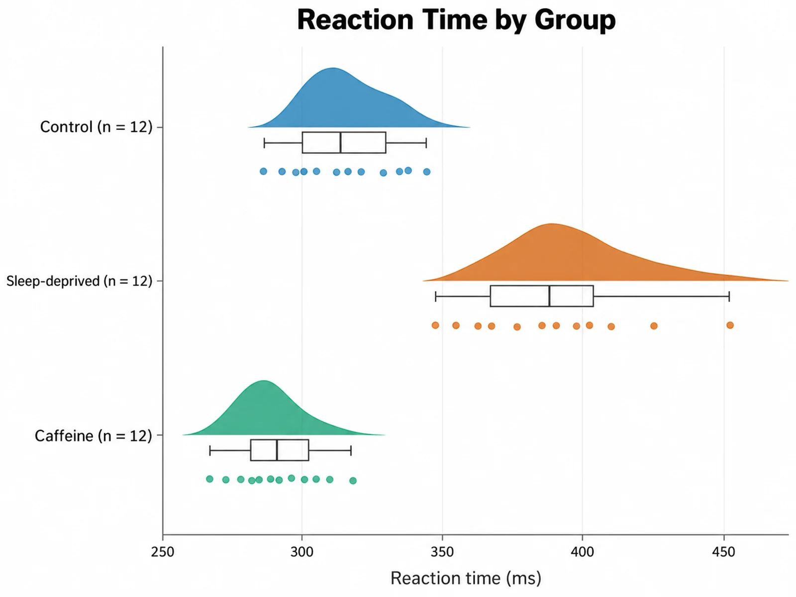
  • For two to five groups with small samples, show the raw points instead, with a raincloud plot or a box plot with jittered points.
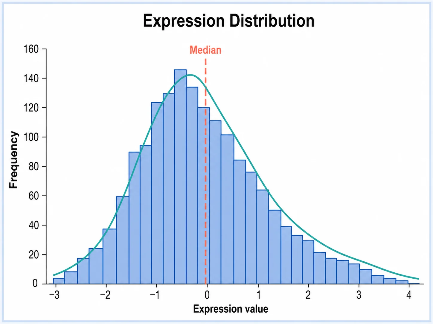
  • For one distribution, a histogram is simpler and shows counts directly.

Ordering, overlap, and color

  • Order: month and weekday names are put in calendar order and numeric labels in numeric order; other groups keep the order they first appear in your file. Write "order by median" (or "by mean, descending") to rank them instead.
  • Overlap: 1.5 to 2 rows of overlap is typical. Ask for "overlap 1" for a calmer plot or "overlap 3" for a dramatic one; too much overlap hides the ridges behind.
  • Color: one color for all ridges is often enough. Use a gradient along the x-axis when the value itself has meaning (temperature), or a sequential palette when the groups are ordered.
  • Overlay: map a third column with two or three levels (control and treated, male and female) to draw semi-transparent overlapping densities inside each ridge.
  • Annotation: median or quartile lines inside each ridge and rug marks for raw values help readers check the curves.

What data does a ridgeline plot need?

  • Long format: one row per observation, with a group column and a numeric value column. Wide tables with one column per group should be reshaped first (for example with pivot_longer in R or melt in pandas).
  • At least 5 values per group are required and 30 or more are recommended; a density curve from a handful of points mostly shows the bandwidth.
  • Up to 20 groups are drawn. Extra groups are listed in a warning so nothing is dropped silently.
  • An optional overlay column can hold up to 3 levels.
  • Uploads are limited to 1,200 rows. For larger datasets, upload a random sample per group.

Ridgeline plot vs violin plot vs box plot

All three compare distributions across groups. They differ in how many groups fit and how much shape they show.

Ridgeline plotViolin plotBox plot
ShowsFull density shapeMirrored density shapeMedian, quartiles, whiskers, outliers
Groups that fit well5 to 302 to 82 to 15
LayoutStacked rows, overlappingSide by sideSide by side
Two peaks visibleYesYesNo
Exact summary valuesOnly if median or quartile lines are drawnUsually with an inner boxYes
Best forMany ordered groups, shifts over timeFew groups, shape plus summaryCompact summaries, outliers

Common ridgeline plot mistakes

Ridgeline plots are easy to make and easy to misread.

  1. MistakeReading a taller ridge as a bigger group.

    CorrectRidge height is density, not count. Print n for each group, because a small, tightly clustered group can have the tallest ridge.

  2. MistakeSmoothing each group with its own bandwidth and comparing the shapes.

    CorrectUse one joint bandwidth so a smoother ridge means a wider distribution, not a different setting.

  3. MistakeDrawing ridges from 6 or 8 points per group.

    CorrectWith small samples, show the raw points with a raincloud or dot plot; a density curve from a few points mostly shows the bandwidth.

  4. MistakeOverlapping the ridges so much that the lower ones disappear.

    CorrectKeep the overlap between about 1 and 2 rows, and use semi-transparent fills with outlines.

  5. MistakeLetting groups appear in random order.

    CorrectOrder by time, dose, or another natural sequence, or by median, so the shift reads from top to bottom.

  6. MistakeTrusting the tails near a hard limit, such as negative reaction times or expression below zero.

    CorrectKernel smoothing spills past the data range. Report medians and quartiles, and mention the limit in the caption.

Ridgeline Plot Maker FAQ

What is a ridgeline plot?

A ridgeline plot is a set of density curves, one per group, stacked vertically on a shared x-axis with a little overlap, so it looks like a mountain range. It shows how the distribution of a variable changes across many groups or over time.

Why are ridgeline plots also called joy plots?

The stacked curves resemble the cover of Joy Division’s 1979 album Unknown Pleasures, so the plots were first called joy plots. In 2017 the author of the R package ggjoy retired the name because of the dark history behind the band’s name, renamed the package ggridges, and the field moved to "ridgeline plot".

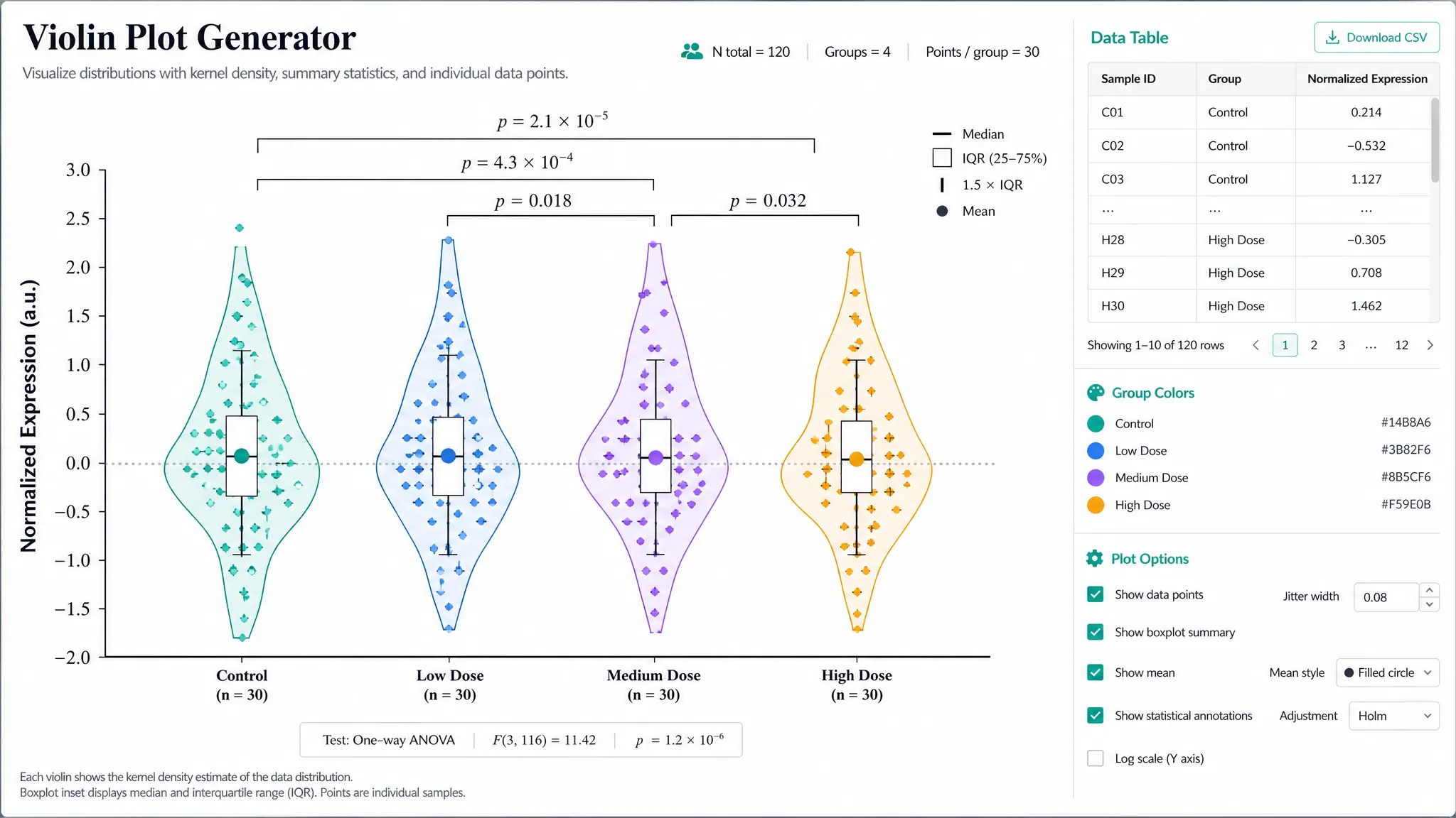
What is the difference between a ridgeline plot and a violin plot?

Both show density shapes. A violin plot mirrors each density and places groups side by side, which works for a handful of groups. A ridgeline plot draws one-sided densities stacked in rows with overlap, which keeps 10 to 20 or more groups readable and makes shifts across ordered groups easy to follow.

How many groups can a ridgeline plot show?

This maker draws up to 20 ridges and lists any extra groups in a warning. Ridgelines stay readable with many groups because each row only needs a little height.

How many data points does each group need?

At least 5 values per group, with 30 or more recommended. With fewer points the curve shape mostly reflects the smoothing bandwidth; show the raw points instead.

What does the height of a ridge mean?

It is the estimated probability density, rescaled so the tallest peak in the whole figure fills one row times the overlap. Heights are comparable between ridges, but they are not counts, and there is no density axis.

How is the smoothing bandwidth chosen?

Each group’s bandwidth is calculated with Silverman’s rule of thumb (R’s bw.nrd0), and their mean is used for every ridge, as ggridges does by default. Ask for "separate bandwidths" to smooth each group on its own.

Can I overlay two conditions in each ridge?

Yes. Map a third column with two or three levels, such as control and treated, as the overlay group. Each ridge then holds semi-transparent overlapping densities, one per level, with a legend.

Can I order the ridges by median?

Yes. Write "order by median" or "order by mean, descending". By default, month and weekday names follow the calendar, numbers sort numerically, and other groups keep their order in your file.

How do I make a ridgeline plot in R or Python?

In R, ggridges provides geom_density_ridges() for ggplot2. In Python, a seaborn FacetGrid with one kdeplot per row, or the joypy package, gives the same layout. This maker does the density estimation for you and returns a finished figure.

Does the AI estimate the curves?

No. The densities, medians, quartiles, and peaks are computed from your rows and passed to the image model as numbers to draw. It does not add statistical tests or p-values. Check the result against your data before publishing.

Ready to compare your distributions?

Generate ridgeline plots, violin plots, raincloud plots, and other distribution figures from your own data with SciFigure AI.