Design Resources
Scientific Color Palettes: How to Choose Colors for Figures, Charts and Posters
Scientific color palettes with HEX codes: qualitative, sequential and diverging schemes, viridis, why to avoid jet, journal palettes and grayscale checks.
 SciFigure AI
Colour in a scientific figure has one job: to carry information the reader can decode correctly. A good palette makes groups easy to tell apart, makes higher values look higher, and still works for a reviewer with red-green colour blindness, on a washed-out projector, and on a page printed in black and white. A bad one invents boundaries that are not in the data or hides a difference that is.
Choosing well comes down to three questions, in this order: what kind of data the colour encodes, how many distinct colours you need, and where the figure will be seen. This guide answers each with ready-to-copy HEX codes for the palettes most used in research figures, the numbers behind them, and what journals actually ask for.
Step 1: Match the palette type to the data
| Data | Palette type | What it looks like | Use for | Good choices |
|---|---|---|---|---|
| Unordered groups | Qualitative (categorical) | Distinct hues of similar weight | Genotypes, treatments, cell types, lines on a plot | Okabe-Ito, Paul Tol bright or muted, IBM |
| Ordered values, low to high | Sequential | One direction of steadily changing lightness | Expression, concentration, density, intensity | viridis, cividis, magma, mako, batlow |
| Values around a meaningful midpoint | Diverging | Two hues meeting at a light neutral centre | Fold change, correlation, anomalies, z-scores | Tol BuRd or sunset, ColorBrewer RdBu, vik |
| Values that wrap around | Cyclic | Starts and ends on the same colour | Angles, phase, time of day, wind direction | twilight (matplotlib), romaO (Crameri) |
Mixing these up is the most common colour error in research figures. A qualitative palette on ordered data makes the reader memorise a legend instead of reading a gradient; a sequential palette on data with a meaningful zero hides which values are above it and which below.
Qualitative palettes: colours for groups
These are the categorical palettes designed with colour-vision deficiency in mind. Each list is in its author's order and was checked against the original source (see Sources).
Okabe-Ito (8 colours, also called the Wong palette). The usual default for lines, points and bars. Our Okabe-Ito palette reference has the RGB values, the best order and code for every major tool.
#000000 #E69F00 #56B4E9 #009E73 #F0E442 #0072B2 #D55E00 #CC79A7
Paul Tol bright (7 colours including grey). Tol's recommended default for qualitative data.
#4477AA #EE6677 #228833 #CCBB44 #66CCEE #AA3377 #BBBBBB
Paul Tol muted (9 colours, plus pale grey #DDDDDD for missing data). For when you need more categories.
#CC6677 #332288 #DDCC77 #117733 #88CCEE #882255 #44AA99 #999933 #AA4499
Paul Tol high-contrast (3 colours). Built to stay distinct in grayscale; the best choice for two or three groups in a figure that may be printed.
#004488 #DDAA33 #BB5566
IBM colour-blind safe (5 colours). Saturated, good on screens and slides.
#648FFF #785EF0 #DC267F #FE6100 #FFB000
All five are in the colorblind-friendly palette tool, with deuteranopia, protanopia and tritanopia previews and one-click code for matplotlib, ggplot2, MATLAB and CSS.
What the default colours get wrong
Software defaults were not chosen for colour-blind readers. We ran each palette through the Machado et al. colour-vision simulation and measured the smallest colour difference (CIEDE2000, ΔE) between any two of its colours. Values below about 5 mean two groups are hard to tell apart; below 2 they are nearly identical.
| Palette | Smallest difference, deuteranopia | Smallest difference, protanopia | Smallest difference, grayscale |
|---|---|---|---|
| matplotlib default (tab10) | 3.4, orange vs olive | 1.4, orange vs green | 1.2, blue vs red |
| ggplot2 default, 3 groups | 5.9, red vs green | 18.1 | 0.3, red vs blue |
| Okabe-Ito, 7 colours without black | 11.5, orange vs yellow | 12.3, blue vs reddish purple | 0.6, orange vs sky blue |
| Tol high-contrast | 25.5 | 26.1 | 17.8 |
Two lessons follow. The defaults are risky for red-green colour blindness, which affects about 1 in 12 men and 1 in 200 women of Northern European ancestry. And no multi-hue palette survives grayscale on its own: even Okabe-Ito's orange and sky blue print as the same grey. Only a palette designed for lightness differences, such as Tol's high-contrast set, does.
Sequential palettes: viridis and the perceptually uniform family
For continuous data, the palette must change lightness steadily from one end to the other, so that equal steps in the data look like equal steps in colour and the order survives in grayscale. Palettes built this way are called perceptually uniform.
viridis was designed by Nathaniel Smith and Stéfan van der Walt for matplotlib, where it became the default colormap in version 2.0. Its siblings magma, inferno and plasma use different hue paths with the same properties, and cividis (Nuñez et al., 2018) was optimised to look almost the same to people with red-green colour blindness. The R package viridisLite adds rocket and mako, two perceptually uniform maps that originated in the seaborn library, plus turbo (see below).
Measured in CIELAB lightness (L*, 0 = black, 100 = white), viridis climbs smoothly from 15 to 91 across ten evenly spaced stops, and cividis from 14 to 91. That steady climb is why both still read correctly in a black-and-white printout.
Ten evenly spaced stops, from matplotlib's colormap data:
viridis  #440154 #482878 #3E4A89 #31688E #26828E #1F9E89 #35B779 #6CCD5A #B5DE2B #FDE725
cividis  #00224E #123570 #3C4A6C #575D6D #707173 #8A8678 #A59C74 #C2B369 #E1CC55 #FEE838
Use the colormap itself in code rather than these stops, so the software interpolates all 256 entries:
import matplotlib.pyplot as plt
plt.imshow(data, cmap="viridis")   # or "cividis", "magma", "inferno", "plasma"

import seaborn as sns
sns.heatmap(df, cmap="mako")       # seaborn's rocket and mako
library(ggplot2)
ggplot(df, aes(x, y, fill = value)) +
  geom_tile() +
  scale_fill_viridis_c(option = "mako")   # "viridis", "cividis", "magma", "rocket", ...
The heatmap generator applies these scales to your own data, and the guide on how to make a heatmap covers scaling and clustering.
Crameri's Scientific colour maps
Fabio Crameri's Scientific colour maps are a free, versioned suite of perceptually uniform maps (batlow is the best known) designed to be readable by colour-blind readers and in black and white. They cover sequential, diverging, cyclic and categorical data and are available for most plotting software, including Python (the cmcrameri package) and R (the scico package). Crameri, Shephard and Heron's 2020 paper in Nature Communications is the clearest short account of why colour choice changes how data are read.
Diverging palettes: when zero means something
Use a diverging palette when the data have a meaningful centre: log fold change, a correlation coefficient, a temperature anomaly, a z-score. Two hues run out from a light, neutral middle, so the eye reads "above" and "below" at once.
Tol BuRd (9)     #2166AC #4393C3 #92C5DE #D1E5F0 #F7F7F7 #FDDBC7 #F4A582 #D6604D #B2182B
Tol sunset (11)  #364B9A #4A7BB7 #6EA6CD #98CAE1 #C2E4EF #EAECCC #FEDA8B #FDB366 #F67E4B #DD3D2D #A50026
Three rules make a diverging scale honest:
- Put the neutral colour at the real midpoint (0 for correlations, 1 for a ratio, 0 for log fold change), not at the middle of your data range.
- Make the limits symmetric (−2 to +2, not −1 to +3) so equal colour intensity means equal distance from the centre.
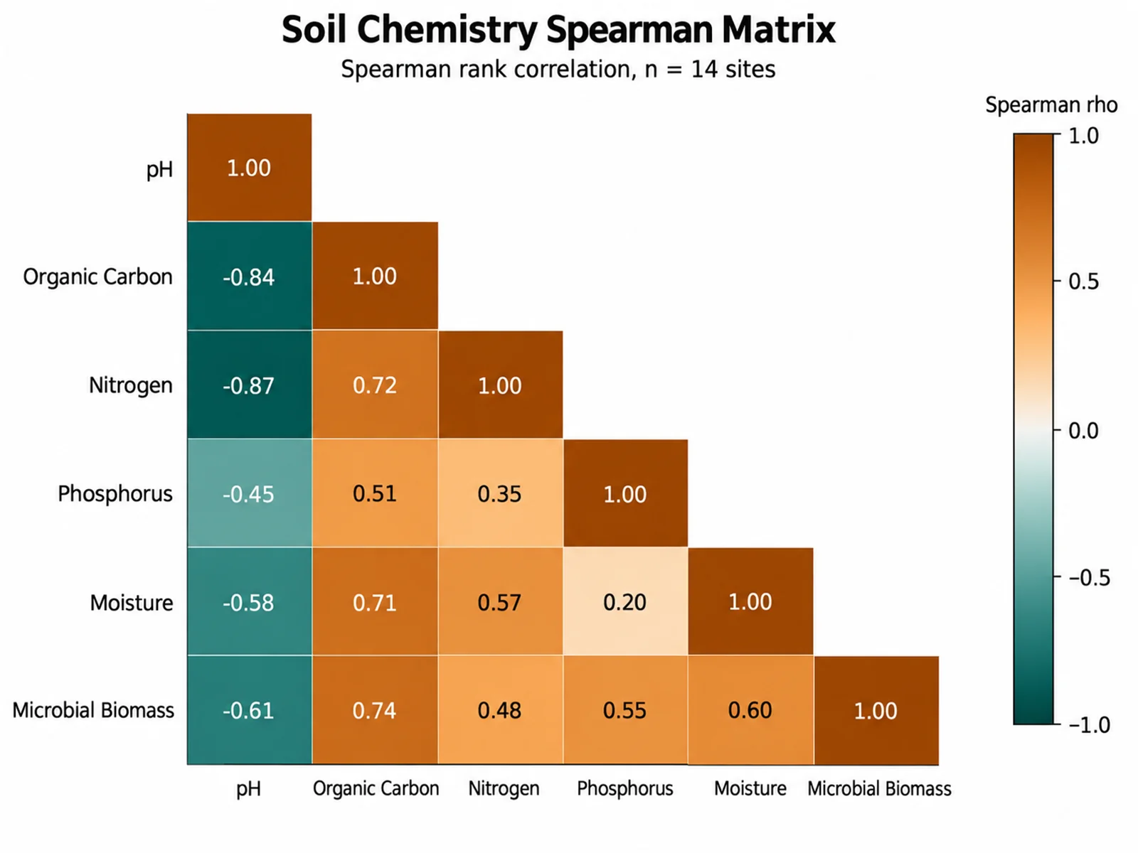
- Prefer blue–red, blue–orange or purple–green over red–green. Tol's BuRd is a reversed ColorBrewer RdBu, and the ColorBrewer diverging schemes (RdBu, BrBG, PuOr) are all safe choices; the cover image of this post uses a brown–teal BrBG-style scale for a correlation matrix.
The correlation matrix generator centres its diverging scale at zero automatically.
Why to avoid rainbow and jet
The rainbow colormap, and its MATLAB-era version jet, is still common in published figures. It misleads in four ways:
- Its lightness goes up and then down. Yellow and cyan in the middle are far lighter than the dark blue and dark red at the ends, so the middle of the range looks like a peak.
- It creates boundaries that are not in the data. The eye sees sharp bands where the hue changes quickly (around yellow and cyan) and flat regions where it changes slowly (the long green stretch).
- It fails for red-green colour blindness, which removes the very hue differences the map depends on.
- It fails in grayscale: low and high values print as the same dark grey.
Borland and Taylor made this case in 2007 and Crameri and colleagues repeated it with examples in 2020. Google's turbo is a smoother rainbow that fixes the banding, but its lightness still rises and falls, so keep it for cases where you need fine detail on screen and say so in the legend. For anything ordered, use a sequential map from the section above.
Journal colour palettes: what Nature, Science and IEEE ask for
People search for a "Nature color palette" expecting a house style. There isn't one. Nature's figure guide asks authors to use an accessible colour palette, citing Bang Wong's 2011 Nature Methods column (the Okabe-Ito colours) as an example, to avoid colour combinations that colour-blind readers cannot distinguish, and to avoid coloured text, using black labels with colour keys instead. It also asks for figures in RGB.
The "journal palettes" you see online come from the R package ggsci, whose palettes are described as inspired by the colours in figures from each journal. They are not official and not designed for colour-blind readers:
| ggsci palette | Inspired by | First colours |
|---|---|---|
npg | Nature Reviews Cancer | #E64B35 #4DBBD5 #00A087 #3C5488 #F39B7F #8491B4 #91D1C2 #DC0000 #7E6148 #B09C85 |
aaas | Science | #3B4992 #EE0000 #008B45 #631879 #008280 #BB0021 #5F559B #A20056 #808180 #1B1919 |
nejm | The New England Journal of Medicine | #BC3C29 #0072B5 #E18727 #20854E #7876B1 #6F99AD #FFDC91 #EE4C97 |
lancet | Lancet Oncology | #00468B #ED0000 #42B540 #0099B4 #925E9F #FDAF91 #AD002A #ADB6B6 #1B1919 |
In our simulation, the full npg set contains two reds that are similar even with normal vision (#E64B35 and #DC0000, ΔE 9.3) and a green and a beige that nearly merge under protanopia (ΔE 4.1); aaas has pairs below ΔE 5 under all three simulated deficiencies. If you like a journal look, use only the first three or four colours and check them in the colorblind simulator before you submit.
IEEE publishes colour figures in colour online at no charge, while colour in the printed journal is a paid option. Figures that rely on hue alone can therefore lose meaning in print, which is one more reason to vary lightness and marker shape. Our journal figure requirements page collects the technical rules (sizes, resolution, file types) by journal.
How many colours can one palette carry?
| Palette | Colours |
|---|---|
| Tol high-contrast | 3 |
| IBM colour-blind safe | 5 |
| Tol bright, Tol vibrant | 7 (including grey) |
| Okabe-Ito | 8 (including black) |
| Tol muted | 9 |
| ColorBrewer Paired and Set3 | 12 |
Readers can reliably match about six to eight colours to a legend, and fewer is faster. Tol notes that beyond nine distinct colours a categorical scheme stops working and suggests switching to a banded or rainbow-style sequential scheme. With more groups than that:
- Split the plot into small multiples, one panel per group, all in the same neutral colour.
- Highlight the few groups that matter in colour and draw the rest in light grey.
- Label lines and regions directly instead of relying on a legend.
- Add a second channel: marker shape, line style or hatching.
Check grayscale and contrast before you export
Two quick numerical checks catch most problems.
Contrast against the background. The Web Content Accessibility Guidelines (WCAG 2.1) ask for a contrast ratio of at least 3:1 for graphical objects such as lines and markers, and 4.5:1 for normal-size text. Light palette colours fail on white:
| Colour on white | Contrast ratio | Thin lines and small markers |
|---|---|---|
| Okabe-Ito yellow #F0E442 | 1.32:1 | Too faint; use only as a fill with a dark outline |
| Okabe-Ito orange #E69F00 | 2.25:1 | Below 3:1; use thicker lines or larger markers |
| Okabe-Ito sky blue #56B4E9 | 2.31:1 | Below 3:1; use thicker lines or larger markers |
| Okabe-Ito reddish purple #CC79A7 | 3.06:1 | Passes 3:1 |
| Okabe-Ito bluish green #009E73 | 3.42:1 | Passes 3:1 |
| Okabe-Ito vermilion #D55E00 | 3.87:1 | Passes 3:1 |
| Okabe-Ito blue #0072B2 | 5.19:1 | Passes, and is dark enough for text |
Grayscale. Convert the finished figure to grayscale, or use the grayscale mode in the colorblind simulator, and check that every group, bar and line can still be told apart. If two cannot, change the lightness of one, or add a shape, pattern or direct label.
Our earlier guide to colorblind-safe palettes for science figures covers redundant encoding in more depth.
A colour palette for research posters
Posters are read from two metres away under conference-hall lighting, so restraint matters more than on a screen.
- Background: white or a very light neutral. Dark backgrounds make photographs and data colours harder to judge.
- Structure colour: one muted accent for headers and boxes, used consistently. Keep it different from your data colours so it never looks like data.
- Data colours: the same qualitative palette in every panel, with each group keeping its colour throughout, and a sequential map for any heatmap.
- Text: black or near-black. Coloured text is hard to read at a distance and, as Nature's guide notes, inaccessible.
The scientific poster maker builds a layout you can drop these colours into, and our font guide for figures and posters covers the type.
Apply a palette in R, Python and spreadsheets
# ggplot2: a categorical palette
pal <- c("#0072B2", "#E69F00", "#009E73", "#D55E00")
ggplot(df, aes(x, y, colour = group)) + geom_point() +
  scale_colour_manual(values = pal)

# ggplot2: a diverging scale centred on zero
ggplot(df, aes(x, y, fill = log2fc)) + geom_tile() +
  scale_fill_distiller(palette = "RdBu", limits = c(-2, 2), oob = scales::squish)
import matplotlib.pyplot as plt
from cycler import cycler

plt.rcParams["axes.prop_cycle"] = cycler(color=["#0072B2", "#E69F00", "#009E73", "#D55E00"])
plt.imshow(log2fc, cmap="RdBu_r", vmin=-2, vmax=2)   # diverging, symmetric limits
In Excel, PowerPoint and GraphPad Prism, set the colours once as a theme or colour scheme rather than recolouring each chart; the Okabe-Ito guide gives the exact menu steps. Our bar chart generator and other chart tools apply accessible palettes for you.
Checklist before you submit
- The palette type matches the data: qualitative, sequential, diverging or cyclic.
- No rainbow or jet on ordered data.
- Six to eight colours at most per panel; more groups are split, greyed out or labelled directly.
- The figure reads correctly under deuteranopia and protanopia simulation.
- The figure reads correctly in grayscale.
- Thin lines and small markers have at least 3:1 contrast against the background.
- Each group keeps the same colour in every panel and figure.
- Labels and legend text are black, not coloured.
Frequently asked questions
What is the best color palette for scientific figures?
For groups, Okabe-Ito or Paul Tol's bright scheme. For continuous data, viridis or cividis. For data around a meaningful zero, a blue–red diverging scheme such as Tol's BuRd. All of them are designed to stay readable for colour-blind readers.
What colours does the viridis palette use?
It runs from dark purple (#440154) through blue and teal to bright yellow (#FDE725), increasing steadily in lightness. Ten evenly spaced stops are listed above; in code, use the built-in viridis colormap rather than the stops.
What is the mako color palette?
A perceptually uniform sequential colormap from the seaborn library that runs from near-black through blue to pale green-blue. It is available in seaborn as "mako" and in R's viridisLite and ggplot2 viridis scales as option "mako" (or "G").
Is there an official Nature journal color palette?
No. Nature asks for an accessible palette, citing the Wong (Okabe-Ito) colours as an example, and asks authors to avoid colour combinations that colour-blind readers cannot distinguish. The "npg" palette in the ggsci R package is only inspired by figures in a Nature journal.
Why is the jet or rainbow colormap bad for science?
Its lightness rises and falls, so it creates false peaks and sharp bands that are not in the data, it relies on red-green differences, and it cannot be read in grayscale. Use viridis, cividis or another perceptually uniform map instead.
How many colors should a chart have?
As few as the data allow, and rarely more than six to eight in one panel. Beyond that, use small multiples, grey out the less important groups, or label lines directly.
How do I make a figure that works in black and white?
Choose colours that differ in lightness, not just hue (Tol's high-contrast scheme is designed for this), and add marker shapes, line styles or hatching. Then convert the figure to grayscale and check every group is still distinguishable.
Which colours should never be used together?
Red with green is the most problematic pair for colour-blind readers. Also avoid pairs of very similar lightness when the figure may be printed in grayscale, and light colours such as yellow for thin lines or text on a white background.
Related guides and tools
- Okabe-Ito color palette: HEX codes and how to use it
- Colorblind-safe palettes for science figures
- Colorblind-friendly palette: every palette in this guide with CVD previews and copy-ready code.
- Colorblind simulator: check your own figure under each type of colour blindness and in grayscale.
- Heatmap generator, correlation matrix generator and bar chart generator.
Sources
- Okabe, M. & Ito, K. Color Universal Design (CUD): How to make figures and presentations that are friendly to colorblind people. 2002, revised 2008.
- Wong, B. (2011). Points of view: Color blindness. Nature Methods, 8, 441.
- Tol, P. Colour schemes and templates: the bright, high-contrast, muted, BuRd and sunset schemes.
- IBM Design Language, Color library: colour-blind safe palette (archived page).
- matplotlib, Choosing colormaps in Matplotlib and the colormap data for viridis and cividis.
- Garnier, S. et al. viridisLite: colorblind-friendly color maps, options A to H including rocket and mako.
- Nuñez, J. R., Anderton, C. R. & Renslow, R. S. (2018). Optimizing colormaps with consideration for color vision deficiency to enable accurate interpretation of scientific data. PLOS ONE, 13(7), e0199239.
- Crameri, F., Shephard, G. E. & Heron, P. J. (2020). The misuse of colour in science communication. Nature Communications, 11, 5444. Crameri, F. Scientific colour maps.
- Borland, D. & Taylor, R. M. (2007). Rainbow color map (still) considered harmful. IEEE Computer Graphics and Applications, 27(2), 14–17.
- Harrower, M. & Brewer, C. A. (2003). ColorBrewer.org: an online tool for selecting colour schemes for maps. The Cartographic Journal, 40(1), 27–37.
- Xiao, N. ggsci: scientific journal and sci-fi themed color palettes for ggplot2 (palette definitions in
R/palettes.R). - Nature Research, Preparing figures: our specifications: accessible palettes, RGB, and coloured text.
- IEEE Author Center, About potential article processing charges: online colour and print colour charges.
- W3C, Web Content Accessibility Guidelines (WCAG) 2.1: success criteria 1.4.3 (text contrast) and 1.4.11 (non-text contrast).
- MedlinePlus Genetics, Color vision deficiency: how common red-green colour blindness is.
- Machado, G. M., Oliveira, M. M. & Fernandes, L. A. F. (2009). A physiologically-based model for simulation of color vision deficiency. IEEE Transactions on Visualization and Computer Graphics, 15(6), 1291–1298.