
Free statistics tool
Bell curve generator with shaded areas and z-scores
Enter a mean and a standard deviation and this bell curve generator draws the normal distribution, shades the region you choose, and reports the exact probability, the z-scores, and the percentile of each bound. Download the result as PNG or SVG for a report, a slide, or a problem set.
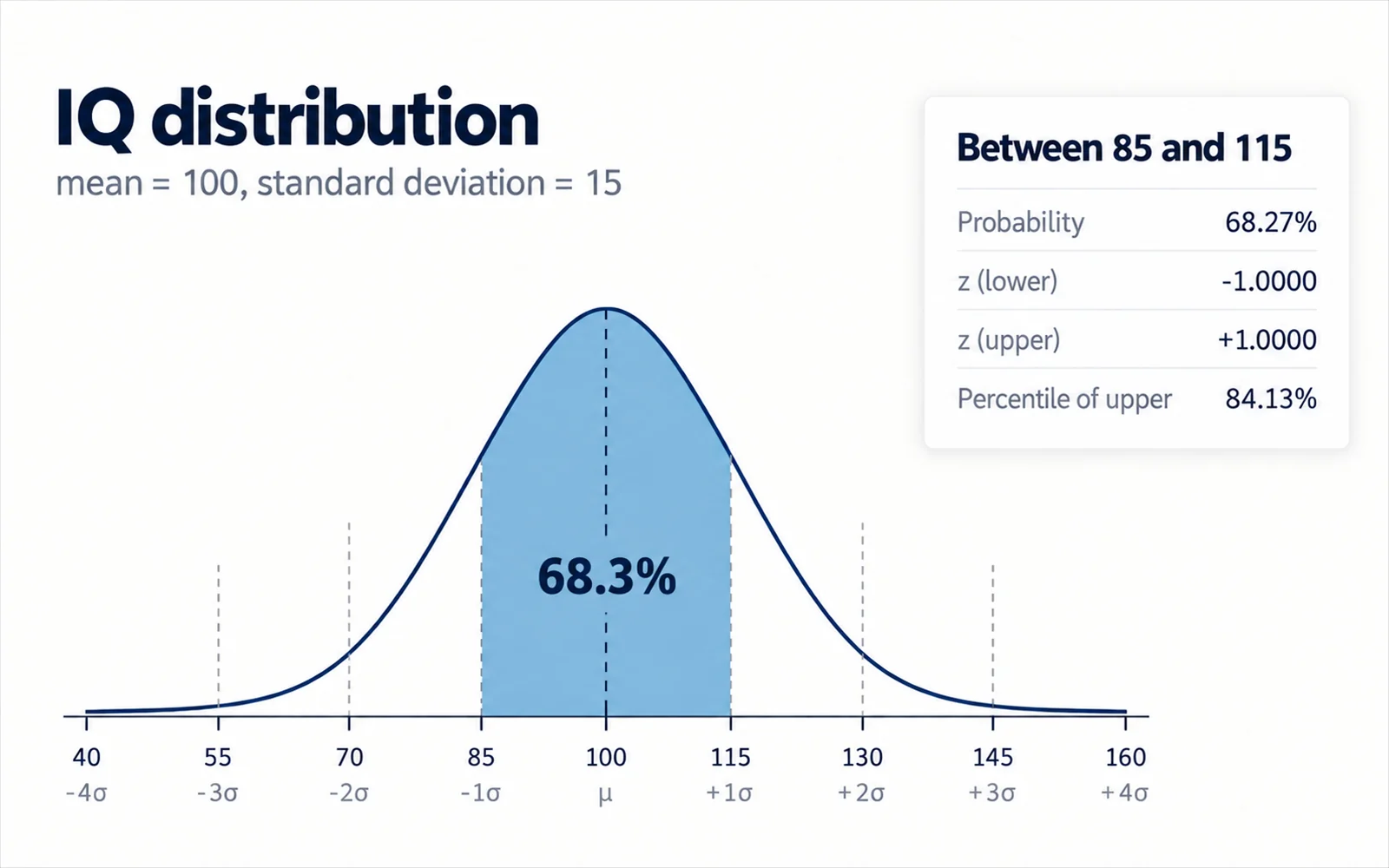
68.27%
of values fall between 85 and 115
- z (lower)
- -1.0000
- z (upper)
- 1.0000
- Percentile of lower
- 15.87%
- Percentile of upper
- 84.13%
How to make a bell curve
A bell curve is the graph of a normal distribution. Two numbers define it completely: the mean, which fixes where the peak sits, and the standard deviation, which fixes how wide the curve spreads. Everything else follows.
- Enter the mean (μ). The curve is symmetric about it, so the mean is also the median and the mode.
- Enter the standard deviation (σ). A larger σ makes the curve flatter and wider; a smaller σ makes it taller and narrower. The total area stays 1 either way.
- Choose what to shade: between two values, below a value, above a value, or both tails.
- Read the percentage. It is the area under the curve in the shaded region, which is the probability a random value falls there.
- Use the central interval buttons to jump straight to the middle 68%, 90%, 95%, or 99% of the distribution.
The 68-95-99.7 rule
The empirical rule states roughly how much of a normal distribution lies within one, two, and three standard deviations of the mean. The tool computes the exact figures rather than the rounded ones, which is why the numbers below are not quite 68, 95, and 99.7.
- Within ±1σ: 68.27% of values. For IQ scores with μ = 100 and σ = 15, that is the range 85 to 115.
- Within ±2σ: 95.45% of values, or 70 to 130 on the same IQ scale.
- Within ±3σ: 99.73% of values, or 55 to 145.
- The familiar "95%" interval is actually ±1.96σ, not ±2σ. At exactly ±1.96σ the area is 95.00%; at ±2σ it is 95.45%.
- The remaining area sits in the tails, split evenly because the curve is symmetric. Beyond ±3σ only 0.27% of values remain.
Z-scores and percentiles
A z-score restates a raw value as the number of standard deviations it sits from the mean, which is what makes two different scales comparable. The formula is z = (x − μ) / σ.
- A z of 0 is the mean. A z of +1.5 is one and a half standard deviations above it; a z of −2 is two below.
- The percentile is the area to the left of a value, so a z of +1 corresponds to the 84.13th percentile.
- Converting between scales means matching z-scores: an IQ of 130 has z = 2, and so does an SAT section score of 700 when μ = 500 and σ = 100.
- Critical values used in hypothesis testing are just z-scores of fixed tail areas: 1.645 for a one-tailed 5% test, 1.960 for a two-tailed 5% test, and 2.576 for a two-tailed 1% test.
When a bell curve is the wrong model
The normal distribution is the default assumption in a great deal of introductory statistics, and it is often a poor one. Drawing a bell curve over data that is not normal hides the thing you most need to see.
- Skewed data. Reaction times, incomes, and concentrations usually have a long right tail. The mean and the median separate, and a symmetric curve misrepresents both.
- Bounded data. Percentages, counts, and proportions cannot go below zero or above their ceiling, so a curve that extends to ±∞ assigns probability to impossible values.
- Small samples. With fewer than about 30 observations, use a t distribution rather than a normal one for confidence intervals and tests.
- Multimodal data. Two overlapping populations produce two peaks, and fitting one bell curve averages them into a shape that describes neither.
- Plot the data first. A histogram, a dot plot, or a Q-Q plot tells you whether a normal model is reasonable before you assume it.
Frequently asked questions
Is this bell curve generator free?
Yes. It runs entirely in your browser, needs no account, and exports PNG and SVG without a watermark. Nothing you enter is uploaded to a server.
What do I need to draw a bell curve?
Just two numbers: the mean and the standard deviation. The mean sets the centre of the curve and the standard deviation sets its width. Everything else, including the height of the peak, follows from those two.
How do I find the percentage between two values?
Set the shade mode to Between, enter the lower and upper bounds, and the tool reports the area under the curve in that range. That area is the probability a randomly drawn value falls between them.
Why is ±2σ 95.45% and not 95%?
Because the round number 95% corresponds to ±1.96σ, not ±2σ. The two are close enough that textbooks often use them interchangeably, but they differ: ±1.96σ gives exactly 95.00% and ±2σ gives 95.45%. Use the 95% central-interval button to get the exact bounds.
What is a z-score?
The number of standard deviations a value sits from the mean, calculated as z = (x − μ) / σ. It lets you compare values measured on different scales, and it is what probability tables are indexed by.
Can I use this for a normal distribution graph in a report?
Yes. Export the SVG for a figure you will edit later, since the text stays live in Illustrator, Inkscape, or PowerPoint, or export the PNG at 1800 pixels wide for a slide or a document.
Does it work with negative means or decimals?
Yes. Any real mean works, including negative values, and both the mean and the standard deviation accept decimals. The standard deviation has to be greater than zero, since a distribution with no spread is not a curve.
Related tools
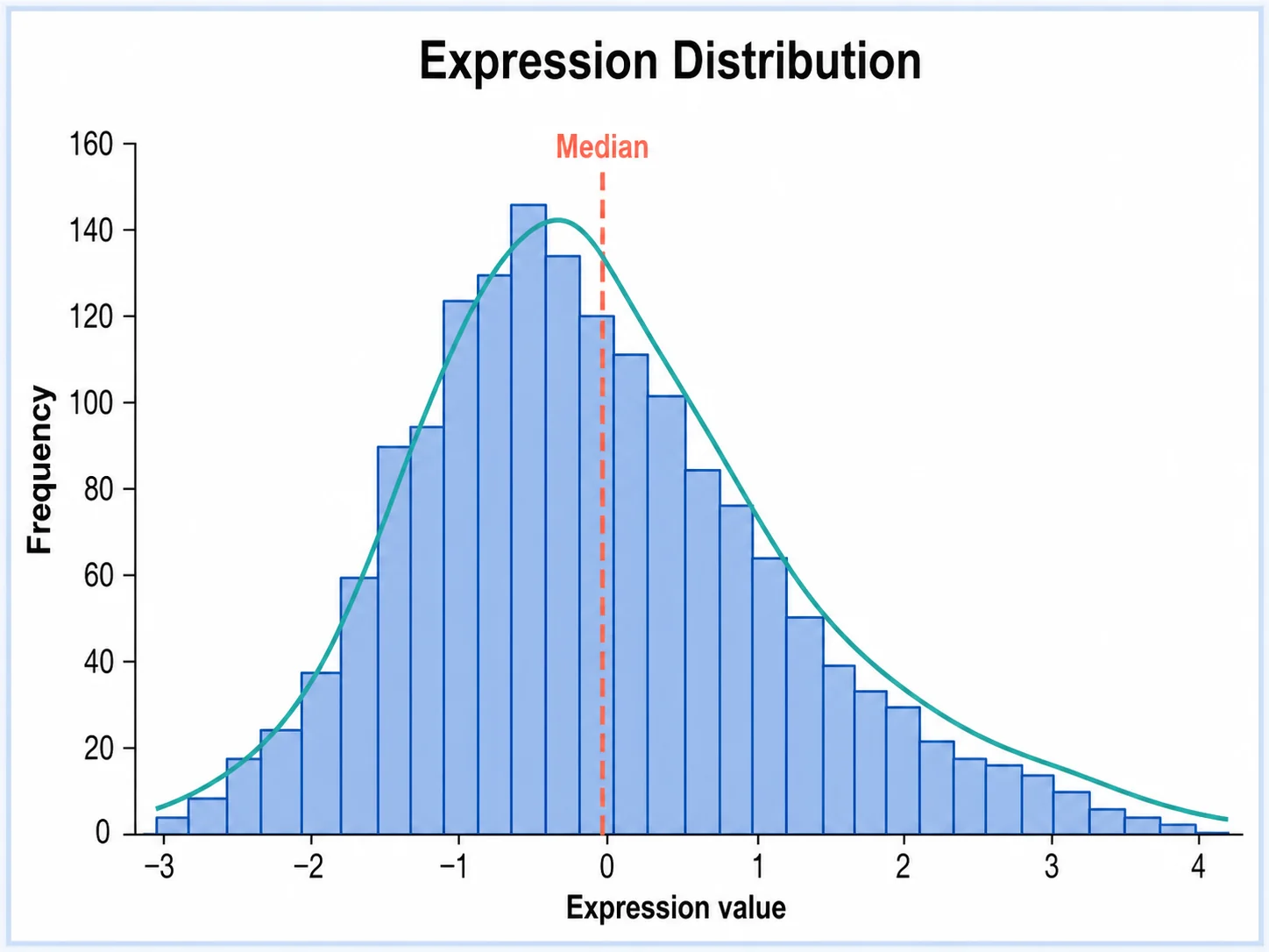
Histogram Generator
Turn a column of values into a publication-ready histogram.
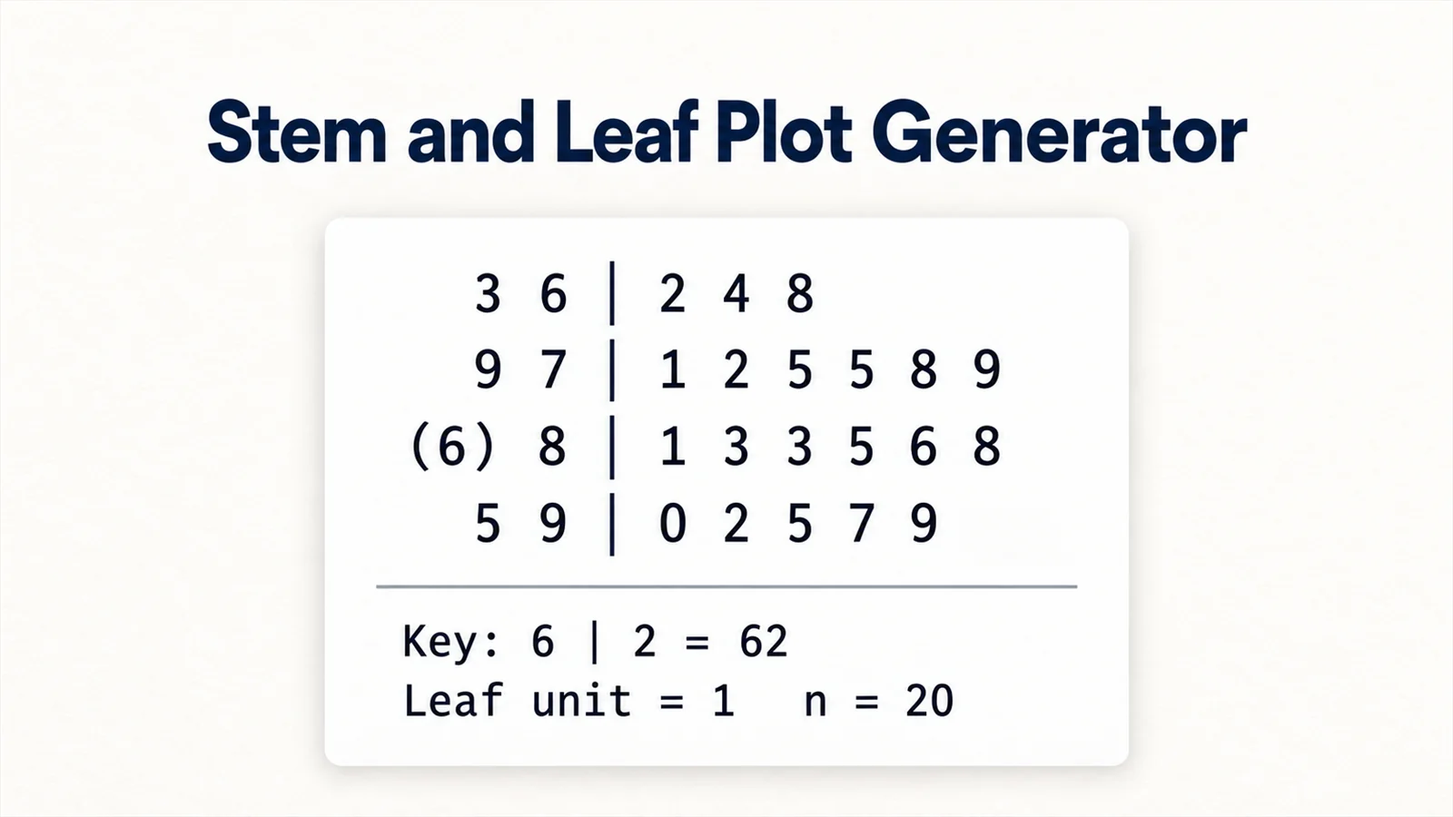
Stem and Leaf Plot Generator
Build a stem-and-leaf display with depths, split stems, and quartiles.

Box Plot Generator
Build box and whisker plots with quartiles and outliers from your own data.
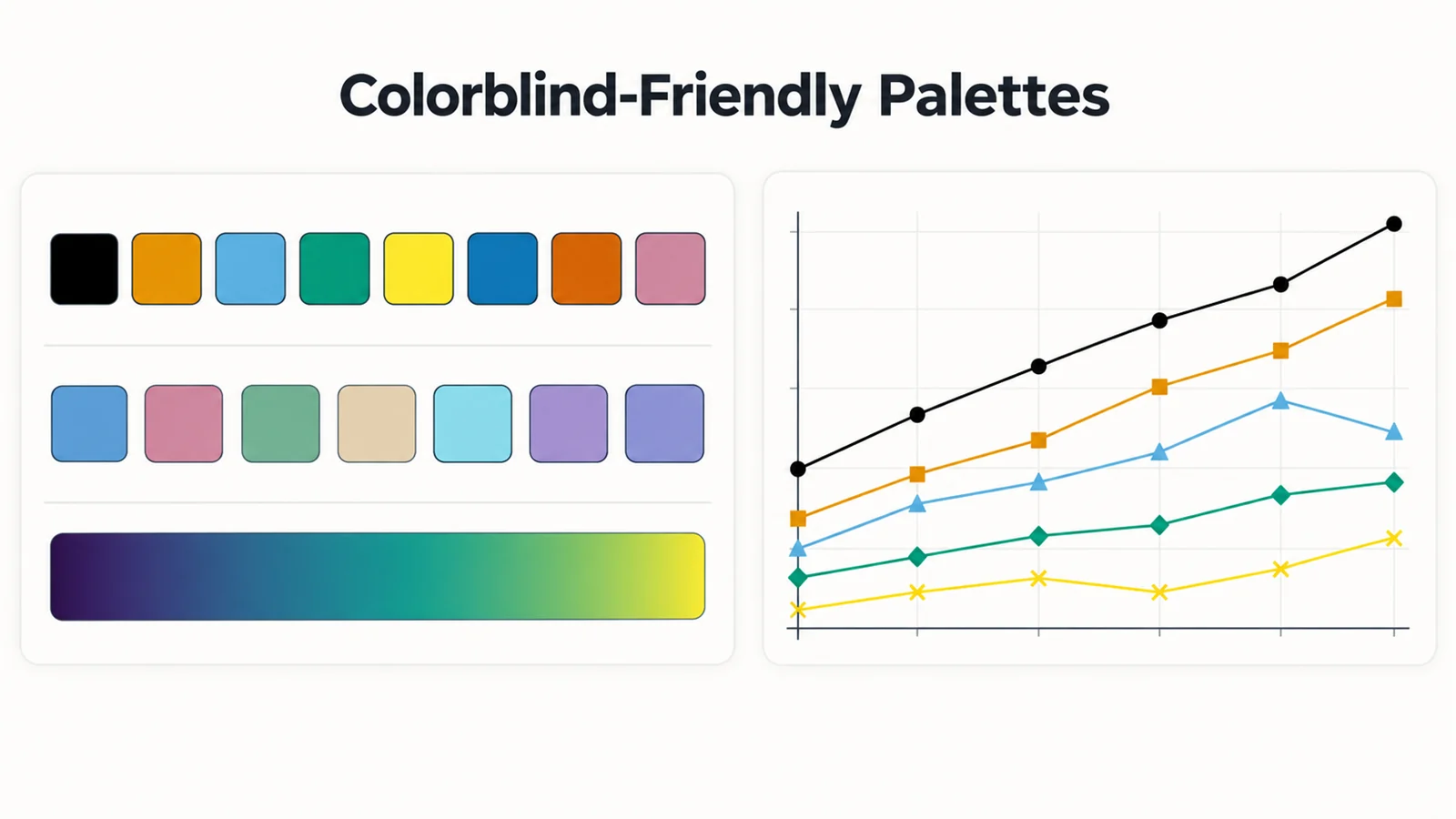
Colorblind-Friendly Palettes
Okabe-Ito and other colorblind-safe palettes with HEX and code snippets.
Need a chart from your own data?
SciFigure AI turns spreadsheets into publication-ready histograms, box plots, and distribution figures for papers and slides.
Explore the chart generatorsLast checked: September 20, 2026. Sources: NIST/SEMATECH e-Handbook: Normal Distribution; Acklam, algorithm for the inverse normal CDF.